

IVF_RABITQ is a Milvus vector index that combines IVF clustering with RaBitQ, a binary quantization method that stores each vector as one bit per dimension and estimates distances with a provable error bound. It compresses FP32 vectors about 32× without training a codebook, and an optional refinement step rescores a shortlist with higher-precision data to push recall above 0.9. It is a strong candidate when IVF_FLAT or IVF_SQ8 no longer fits your memory budget.
This page covers what is specific to RaBitQ and the Milvus parameters. For the general background on scalar, product, residual, and binary quantization, the memory math, and how refiners work across index types, see what is vector quantization.
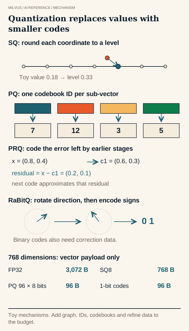 Treat compression as another approximation
How does RaBitQ work?
RaBitQ was introduced by Jianyang Gao and Cheng Long at SIGMOD 2024. Its goal was to keep the extreme compression of 1-bit codes while fixing the main weakness of naive binarization: plain sign bits discard so much information that distance estimates become unreliable. RaBitQ gets there with three ideas.
1. Encode direction relative to a centroid. In IVF_RABITQ each vector is first assigned to its nearest IVF centroid. RaBitQ then works with the residual (vector minus centroid), normalized to unit length. The code therefore captures the direction of the vector from its cluster center, and the length is kept separately as a scalar.
2. Randomly rotate, then take one bit per dimension. The normalized residual is multiplied by a random orthogonal matrix before quantization. The rotation spreads information evenly across coordinates so no single dimension dominates, which is what makes a sign-like 1-bit code informative. The Milvus implementation shows this as an RR({dim}) (random rotation) stage in its FAISS factory string, followed by IVF{nlist},RaBitQ. A D-dimensional vector becomes a D-bit string, so a 768-dimensional vector takes 96 bytes instead of 3,072.
3. Estimate distances with a corrected, unbiased estimator. Next to each code, RaBitQ stores a couple of precomputed per-vector constants. At query time the query stays at full precision, and the squared distance is estimated as the sum of the vector’s distance to its centroid, the query’s distance to that centroid, and a correction term built from the inner product between the binary code and the query residual. With a full-precision query, that inner product combines binary code signs with floating-point query values; it does not reduce to popcount alone. The optional query-quantization path (rbq_query_bits from 1 to 8) enables bitwise acceleration using popcount. The paper proves the estimator is unbiased and gives an error bound that tightens as dimension grows, which suits the 512 to 4096 dimensional embeddings common today.
How is RaBitQ different from PQ and plain binary quantization?
| Product quantization (PQ) | Naive binary (sign bits) | RaBitQ | |
|---|---|---|---|
| Bits per dimension | m × nbits / D, tunable | 1 | 1 |
| Codebook training | k-means per subspace | None | None (random rotation) |
| Distance computation | Lookup table per query | Hamming distance | Corrected inner product; popcount fast path with quantized queries |
| Error guarantee | Empirical only | None | Theoretical bound |
| Sensitivity to data drift | Codebooks can go stale | Low | Low |
The absence of training is operationally useful. A PQ codebook learned on one sample can fit poorly when the corpus or embedding model changes, while RaBitQ’s rotation is data-independent. The authors later published an extended RaBitQ that uses several bits per dimension to trade more space for accuracy; Milvus’s IVF_RABITQ uses the 1-bit code and gets extra accuracy from its refinement step instead.
IVF_RABITQ parameters in Milvus
IVF_RABITQ is available in Milvus 2.6.x and 3.0.x and supports the L2, IP, and COSINE metrics.
Build parameters
| Parameter | Default | Range | What it controls |
|---|---|---|---|
nlist | 128 | 1–65536 | Number of k-means clusters. Docs suggest 32–4096. |
refine | false | true / false | Store a higher-precision copy for rescoring. Recommended when you need 0.9+ recall. |
refine_type | none | SQ6, SQ8, FP16, BF16, FP32 | Precision of the refinement copy. Listed in order of rising recall and storage, falling QPS; SQ8 is the suggested start. |
Search parameters
| Parameter | Default | Range | What it controls |
|---|---|---|---|
nprobe | 8 | 1–nlist | Clusters scanned per query. Higher means better candidate coverage and more latency. |
rbq_query_bits | 0 | 0–8 | Optional scalar quantization of the query. 0 keeps the query at full precision (best recall, slowest). The docs suggest testing 0, 8, and 6, which give similar recall with 6 fastest. |
refine_k | 1 | ≥1 | Candidate magnification for refinement: Milvus picks limit × refine_k candidates with RaBitQ, then reranks them with the refinement data. |
index_params = client.prepare_index_params()
index_params.add_index(
    field_name="embedding",
    index_type="IVF_RABITQ",
    metric_type="COSINE",
    params={"nlist": 1024, "refine": True, "refine_type": "SQ8"},
)
client.create_index("docs", index_params)

results = client.search(
    collection_name="docs",
    data=[query_vec],
    limit=10,
    search_params={"params": {"nprobe": 64, "rbq_query_bits": 0, "refine_k": 2}},
)
Performance depends heavily on fast popcount. The Milvus docs call out CPUs with the AVX512VPOPCNTDQ instruction set (Intel Ice Lake and later, AMD Zen 4 and later); benchmark on the instance type you will deploy.
What does the memory budget actually look like?
Take 100 million 768-dimensional vectors. The raw FP32 payload is about 307 GB. RaBitQ codes for the same vectors are about 9.6 GB, the 32× headline. But the loaded index also holds centroids, per-vector correction constants, IDs, and, if refine is on, the refinement copy. With refine_type="SQ8" that copy alone is about 77 GB, so the realistic comparison is “IVF_RABITQ + SQ8 refine” versus IVF_SQ8 at roughly the same recall, not 9.6 GB versus 307 GB. The win is that the hot first pass touches only tiny codes, and you can pick a cheaper or more expensive refiner independently. Always measure loaded memory in Milvus rather than multiplying a code ratio across the whole service; the memory estimation guide lists the other components.
How should you evaluate IVF_RABITQ?
A recall problem in IVF_RABITQ can come from three places, and each has its own knob:
- The embedding model decides whether true nearest neighbors are actually relevant. No index setting fixes that.
- IVF candidate selection decides which clusters are scanned. If the right neighbor sits in an unprobed cluster, raise
nprobe(or revisitnlist). - Quantized distance estimation decides how candidates are ordered. If the neighbor was scanned but ranked too low, enable
refine, raiserefine_k, or choose a more preciserefine_type.
A practical procedure:
- Build a
FLATindex on the same field to get exact top-k ground truth. The FLAT baseline article explains why this matters. - Build
IVF_FLAT,IVF_SQ8, and IVF_RABITQ with the samenlist, so IVF coverage is identical and only the representation differs. - Sweep
nprobefirst withrefineoff to see the raw RaBitQ curve, then turn on refinement and sweeprefine_kandrbq_query_bits. - Compare at matched Recall@k, recording p50/p99 latency, QPS, loaded memory, and build time. Include filtered queries and the real
limityour application uses. - Keep per-query failures, not just averages. Rare entities and highly selective filters often degrade first.
Re-run the comparison whenever you change embedding models or the corpus shifts noticeably, since the operating point you chose may move. For a broader look at benchmarking practice, see how to benchmark vector search, and for how IVF partitions the space, see how IVF indexes use centroids.
To try IVF_RABITQ on your own data, start a local instance with the Milvus Quickstart and follow the IVF_RABITQ guide.


