

Milvus is a distributed vector database built as four independent layers: stateless proxies that accept client requests, a single Coordinator that manages metadata and schedules work, three kinds of worker nodes (Streaming Nodes for fresh writes, Query Nodes for historical data, Data Nodes for compaction and index building), and a storage layer made of a metadata store, a write-ahead log, and object storage. Because compute and storage are fully disaggregated, you can scale ingestion, search, and background processing separately, and a worker can be replaced without losing data.
That one paragraph is the architecture in miniature. The rest of this page explains why the pieces are split this way, how a record travels from insert() to a search result, and how the design shows up when you deploy, scale, or debug Milvus.
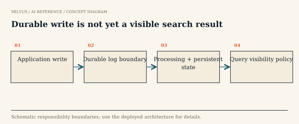 Durable write is not yet a visible search result
What are the four layers of Milvus?
| Layer | Components | What it owns | State |
|---|---|---|---|
| Access | Proxy | Validates requests, routes them to the right shards, merges partial results | Stateless; scale behind a load balancer |
| Coordination | Coordinator | DDL/DCL, timestamp allocation (TSO), binding WAL channels to Streaming Nodes, query topology and load balancing, dispatching compaction and index tasks | One active instance, standby for high availability |
| Worker | Streaming Node, Query Node, Data Node | Real-time writes and fresh data; loading and searching historical segments; offline compaction and index builds | Effectively stateless; rebuildable from storage |
| Storage | Meta store (etcd), WAL storage (Woodpecker by default; Pulsar or Kafka also supported), object storage (S3, MinIO, GCS, Azure Blob) | Schemas and checkpoints; the ordered log of changes; segment data, index files, and log snapshots | Durable source of truth |
The important design choice is that nothing a worker holds is the only copy. Durable state lives in etcd, the WAL, and object storage. Workers cache and compute over it. That is what lets Milvus run on Kubernetes with ordinary rolling restarts and autoscaling, and why the same software can run as one process or as dozens of pods.
How does a write become searchable?
Follow a single insert call:
- Proxy. The client’s request lands on any proxy. The proxy checks the schema, assigns primary keys if
auto_idis on, hashes each row’s primary key to one of the collection’s shards, and gets timestamps from the Coordinator’s timestamp oracle. Each shard maps to a virtual channel (vchannel) in the WAL. - Streaming Node and WAL. The Streaming Node that owns that vchannel appends the rows to the write-ahead log. Once the WAL has durably recorded them, the client gets its acknowledgment. Every DML and DDL operation is a message with a TSO timestamp, so order inside a channel is well defined.
- Growing segment. The Streaming Node also keeps the new rows in an in-memory growing segment and can search it immediately with brute-force or a lightweight interim index. This is why fresh data is queryable long before it is fully indexed.
- Seal and flush. When a growing segment reaches its size or time limit, it is sealed and written to object storage as columnar binlogs.
- Index build and compaction. The Coordinator schedules a Data Node to build the vector and scalar indexes you declared (HNSW, IVF, DiskANN, and so on) on the sealed segment, and to compact small or delete-heavy segments over time.
- Load. Query Nodes load the sealed, indexed segment (or, with tiered storage, just its metadata) and start serving it. The growing copy is then dropped.
The key point: an acknowledged write and a search-visible write are two different events. The acknowledgment means the WAL has it and it will survive a crash. Whether your next search sees it depends on the consistency level you ask for, not on indexing progress.
How does a search request flow through Milvus?
A search reverses the direction. The proxy receives the query vector, filter expression, and limit, then sends it to every shard of the collection (or only the partitions you named). For each shard, a delegator combines two sources: the growing data on the Streaming Node, and the sealed segments spread across Query Nodes. Each Query Node runs the ANN search segment by segment inside Knowhere, the C++ vector engine, applying the scalar filter as a bitset so excluded rows never enter the top-k. Partial results are reduced per node, per shard, and finally at the proxy, which returns the global top-k with the requested output fields.
Two consequences matter for application design:
- Latency is the slowest shard plus the merge. Adding Query Nodes spreads segments thinner and lowers per-node work; adding replicas lets independent copies serve more concurrent queries. They solve different problems (see sharding vs. replication).
- Freshness is a per-request choice. Milvus attaches a guarantee timestamp to each search. With
Strong, the query waits until all data up to “now” is visible. The default,Bounded, tolerates a short lag in exchange for lower latency;Sessionguarantees you see your own writes;Eventuallyskips the wait entirely. The eventual consistency explainer covers when each makes sense.
Why separate streaming, query, and data nodes?
The three worker roles have very different resource profiles, so splitting them is about not letting one workload starve another:
- Streaming Nodes are latency-sensitive and write-heavy. They own WAL appends, shard-level consistency, recovery after restart, and queries over growing data.
- Query Nodes are memory-, disk-, and CPU-heavy. Their job is to keep historical segments and indexes close to compute and run ANN traversal at high concurrency.
- Data Nodes are bursty batch workers. Index building and compaction can saturate CPU for minutes; isolating them keeps that from inflating query tail latency.
Earlier Milvus 2.x releases split coordination across RootCoord, DataCoord, QueryCoord, and IndexCoord, ran separate Index Nodes, and required an external message queue such as Pulsar or Kafka. Milvus 2.6 merged the coordinators into one Coordinator, introduced the Streaming Node, folded index building into Data Nodes, and made Woodpecker, a WAL that writes directly to object storage with no local disk, the default. Woodpecker can run embedded in the Milvus process or, in Milvus 3.0, as its own scalable service. If a tutorial you are reading mentions IndexCoord or requires Pulsar, it describes the older layout.
Where does Milvus store data?
Everything durable ends up in three places. etcd holds collection schemas, segment metadata, and checkpoints, so it is small but must be highly available. The WAL holds the ordered stream of recent changes until they are flushed. Object storage holds everything large: segment binlogs, delete logs, index files, and snapshots.
Query Nodes do not have to hold all of that in RAM. Index types such as DiskANN keep most of the graph on local NVMe, mmap lets the OS page data in and out, and tiered storage (Milvus 2.6.4 and later) loads only segment metadata at first, fetches field and index chunks on demand, and evicts cold data with an LRU policy. The trade-offs between these are covered in mmap vs. disk-oriented ANN indexes.
Milvus 3.0 adds Storage V3, a manifest-based columnar format implemented by the milvus-storage project, plus point-in-time snapshots and external collections that search Parquet, Lance, Iceberg, or Vortex data in place instead of copying it in.
How do deployment modes map to the architecture?
| Mode | How the layers run | Good for |
|---|---|---|
| Milvus Lite | Embedded in your Python process via MilvusClient("./milvus_demo.db"); FLAT index only, no partitions or RBAC | Notebooks, prototypes, tests |
| Standalone | All components in one process (Docker or binary), embedded WAL | Small to medium datasets, single-node production |
| Distributed | Each component is its own pod on Kubernetes, scaled independently | Large datasets, high QPS, high availability |
| Zilliz Cloud | Same architecture operated as a managed service, or in your own cloud account with BYOC | Teams that want Milvus without running it |
The client API is the same across all of them, so code written against Lite moves to a cluster by changing the URI.
What does this mean when you operate Milvus?
The architecture tells you where to look when something is slow:
- New data takes too long to appear in search. Check the write path: WAL append latency, Streaming Node load, and the consistency level you requested. More Query Nodes will not help.
- Search latency climbs during ingestion spikes. Look at growing-segment size and whether index builds are falling behind, which leaves more data to be searched without a proper index.
- Loads are slow or Query Nodes run out of memory. That is segment loading and index footprint: consider DiskANN, mmap, tiered storage, or quantized indexes.
- Query throughput plateaus. Add replicas for concurrency, or Query Nodes if segments per node are the bottleneck.
Measure each stage separately: ingestion acknowledgment, source-to-search freshness, index backlog, and search latency, because each can fail on its own. The bottleneck guide walks through that diagnosis, and Attu gives you a visual view of collections, segments, and load state while you do it.
Related reading
- How do you locate a bottleneck across Milvus components?
- What is Knowhere, and how does Milvus use it?
- What does the milvus-storage project provide?
- How do sharding and replication differ in a vector database?
- How should you compare managed vector databases, BYOC, and self-hosted Milvus?
The fastest way to see the architecture in action is to run the Milvus Quickstart, then deploy Standalone or a cluster when you need more scale. If you would rather not operate the coordinator, workers, and storage yourself, Zilliz Cloud runs the same engine as a managed service.


