Home
Blog
Optimizing NVIDIA CAGRA in Milvus: A Hybrid GPU–CPU Approach to Faster Indexing and Cheaper Queries

Optimizing NVIDIA CAGRA in Milvus: A Hybrid GPU–CPU Approach to Faster Indexing and Cheaper Queries

Engineering

December 10, 2025

Marcelo Chen

As AI systems move from experiments to production infrastructure, vector databases are no longer dealing with millions of embeddings. Billions are now routine, and tens of billions are increasingly common. At this scale, algorithmic choices affect not only performance and recall, but also translate directly into infrastructure cost.

This leads to a core question for large-scale deployments: how do you choose the right index to deliver acceptable recall and latency without letting compute resource usage spiral out of control?

Graph-based indexes such as NSW, HNSW, CAGRA, and Vamana have become the most widely adopted answer. By navigating pre-built neighborhood graphs, these indexes enable fast nearest-neighbor search at billion scale, avoiding brute-force scanning and comparison of every vector against the query.

However, the cost profile of this approach is uneven. Querying a graph is relatively cheap; constructing it is not. Building a high-quality graph requires large-scale distance computations and iterative refinement across the entire dataset—workloads that traditional CPU resources struggle to handle efficiently as data grows.

NVIDIA’s CAGRA addresses this bottleneck by using GPUs to accelerate graph construction through massive parallelism. While this significantly reduces build time, relying on GPUs for both index construction and query serving introduces higher cost and scalability constraints in production environments.

To balance these tradeoffs, Milvus 2.6.1 adopts a hybrid design for GPU_CAGRA indexes: GPUs are used only for graph construction, while query execution runs on CPUs. This preserves the quality advantages of GPU-built graphs while keeping query serving scalable and cost-efficient—making it especially well suited for workloads with infrequent data updates, large query volumes, and strict cost sensitivity.

What Is CAGRA and How Does It Work?

Graph-based vector indexes generally fall into two major categories:

Iterative graph construction, represented by CAGRA (already supported in Milvus).
Insert-based graph construction, represented by Vamana (currently under development in Milvus).

These two approaches differ significantly in their design goals and technical foundations, making each suitable for different data scales and workload patterns.

NVIDIA CAGRA (CUDA ANN Graph-based) is a GPU-native algorithm for approximate nearest neighbor (ANN) search, designed for building and querying large-scale proximity graphs efficiently. By leveraging GPU parallelism, CAGRA significantly accelerates graph construction and delivers high-throughput query performance compared with CPU-based approaches such as HNSW.

CAGRA is built on the NN-Descent (Nearest Neighbor Descent) algorithm, which constructs a k-nearest-neighbor (kNN) graph through iterative refinement. In each iteration, candidate neighbors are evaluated and updated, gradually converging toward higher-quality neighborhood relationships across the dataset.

After each refinement round, CAGRA applies additional graph pruning techniques—such as 2-hop detour pruning—to remove redundant edges while preserving search quality. This combination of iterative refinement and pruning results in a compact yet well-connected graph that is efficient to traverse at query time.

Through repeated refinement and pruning, CAGRA produces a graph structure that supports high recall and low-latency nearest-neighbor search at large scale, making it particularly well suited for static or infrequently updated datasets.

Step 1: Building the Initial Graph with NN-Descent

NN-Descent is based on a simple but powerful observation: if node u is a neighbor of v, and node w is a neighbor of u, then w is very likely a neighbor of v as well. This transitive property allows the algorithm to discover true nearest neighbors efficiently, without exhaustively comparing every pair of vectors.

CAGRA uses NN-Descent as its core graph construction algorithm. The process works as follows:

1. Random initialization: Each node starts with a small set of randomly selected neighbors, forming a rough initial graph.

2. Neighbor expansion: In each iteration, a node gathers its current neighbors and their neighbors to form a candidate list. The algorithm computes similarities between the node and all candidates. Because each node’s candidate list is independent, these computations can be assigned to separate GPU thread blocks and executed in parallel at a massive scale.

3. Candidate list update: If the algorithm finds candidates that are closer than the node’s current neighbors, it swaps out the more distant neighbors and updates the node’s kNN list. Over multiple iterations, this process produces a much higher-quality approximate kNN graph.

4. Convergence check: As iterations progress, fewer neighbor updates occur. Once the number of updated connections drops below a set threshold, the algorithm stops, indicating the graph has effectively stabilized.

Because neighbor expansion and similarity computation for different nodes are fully independent, CAGRA maps each node’s NN-Descent workload to a dedicated GPU thread block. This design enables massive parallelism and makes graph construction orders of magnitude faster than traditional CPU-based methods.

Step 2: Pruning the Graph with 2-Hop Detours

After NN-Descent completes, the resulting graph is accurate but overly dense. NN-Descent intentionally keeps extra candidate neighbors, and the random initialization phase introduces many weak or irrelevant edges. As a result, each node often ends up with a degree two times—or even several times—higher than the target degree.

To produce a compact and efficient graph, CAGRA applies 2-hop detour pruning.

The idea is straightforward: if node A can reach node B indirectly through a shared neighbor C (forming a path A → C → B), and the distance of this indirect path is comparable to the direct distance between A and B, then the direct edge A → B is considered redundant and can be removed.

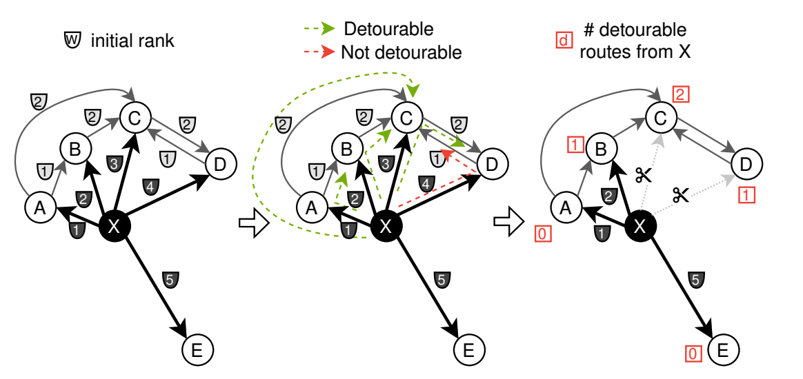
A key advantage of this pruning strategy is that each edge’s redundancy check depends only on local information—the distances between the two endpoints and their shared neighbors. Because every edge can be evaluated independently, the pruning step is highly parallelizable and fits naturally onto GPU batch execution.

As a result, CAGRA can prune the graph efficiently on GPUs, reducing storage overhead by 40–50% while preserving search accuracy and improving traversal speed during query execution.

GPU_CAGRA in Milvus: What’s Different?

While GPUs offer major performance advantages for graph construction, production environments face a practical challenge: GPU resources are far more expensive and limited than CPUs. If both index building and query execution depend solely on GPUs, several operational issues quickly emerge:

Low resource utilization: Query traffic is often irregular and bursty, leaving GPUs idle for long periods and wasting expensive compute capacity.
High deployment cost: Assigning a GPU to every query-serving instance drives up hardware costs, even though most queries do not fully utilize GPU performance.
Limited scalability: The number of GPUs available directly caps how many service replicas you can run, restricting your ability to scale with demand.
Reduced flexibility: When both index building and querying depend on GPUs, the system becomes tied to GPU availability and cannot easily shift workloads to CPUs.

To address these constraints, Milvus 2.6.1 introduces a flexible deployment mode for the GPU_CAGRA index through the adapt_for_cpu parameter. This mode enables a hybrid workflow: CAGRA uses the GPU to build a high-quality graph index, while query execution runs on the CPU—typically using HNSW as the search algorithm.

In this setup, GPUs are used where they deliver the most value—fast, high-accuracy index construction—while CPUs handle large-scale query workloads in a far more cost-effective and scalable manner.

As a result, this hybrid approach is particularly well suited for workloads where:

Data updates are infrequent, so index rebuilds are rare
Query volume is high, requiring many inexpensive replicas
Cost sensitivity is high, and GPU usage must be tightly controlled

Understanding `adapt_for_cpu`

In Milvus, the adapt_for_cpu parameter controls how a CAGRA index is serialized to disk during index building and how it is deserialized into memory at load time. By changing this setting at build time and load time, Milvus can flexibly switch between GPU-based index construction and CPU-based query execution.

Different combinations of adapt_for_cpu at build time and load time result in four execution modes, each designed for a specific operational scenario.

Build Time (`adapt_for_cpu`)	Load Time (`adapt_for_cpu`)	Execution Logic	Recommended Scenario
true	true	Build with GPU_CAGRA → serialize as HNSW → deserialize as HNSW → CPU querying	Cost-sensitive workloads; large-scale query serving
true	false	Build with GPU_CAGRA → serialize as HNSW → deserialize as HNSW → CPU querying	Ensuing queries fall back to the CPU when parameter mismatches occur
false	true	Build with GPU_CAGRA → serialize as CAGRA → deserialize as HNSW → CPU querying	Keeping the original CAGRA index for storage while enabling a temporary CPU search
false	false	Build with GPU_CAGRA → serialize as CAGRA → deserialize as CAGRA → GPU querying	Performance-critical workloads where cost is secondary

Note: The adapt_for_cpu mechanism supports only one-way conversion. A CAGRA index can be converted into HNSW because the CAGRA graph structure preserves all neighbor relationships that HNSW needs. However, an HNSW index cannot be converted back to CAGRA, as it lacks the additional structural information needed for GPU-based querying. As a result, the build-time settings should be selected carefully, with consideration for long-term deployment and querying requirements.

Putting GPU_CAGRA to the Test

To evaluate the effectiveness of the hybrid execution model—using GPUs for index construction and CPUs for query execution—we conducted a series of controlled experiments in a standardized environment. The evaluation focuses on three dimensions: index build performance, query performance, and recall accuracy.

Experimental Setup

The experiments were performed on widely adopted, industry-standard hardware to ensure the results remain reliable and broadly applicable.

CPU: MD EPYC 7R13 Processor(16 cpus)
GPU: NVIDIA L4

1. Index Build Performance

We compare CAGRA built on the GPU with HNSW built on the CPU, under the same target graph degree of 64.

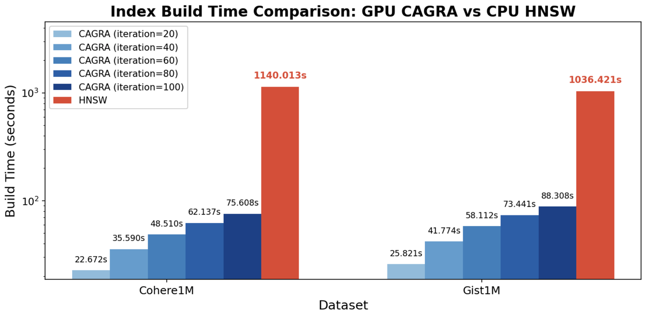
Key Findings

GPU CAGRA builds indexes 12–15× faster than CPU HNSW. On both Cohere1M and Gist1M, GPU-based CAGRA significantly outperforms CPU-based HNSW, highlighting the efficiency of GPU parallelism during graph construction.
Build time increases linearly with NN-Descent iterations. As iteration counts rise, build time grows in a near-linear manner, reflecting the iterative refinement nature of NN-Descent and providing a predictable trade-off between build cost and graph quality.

2. Query performance

In this experiment, the CAGRA graph is built once on the GPU and then queried using two different execution paths:

CPU querying: the index is deserialized into HNSW format and searched on the CPU
GPU querying: search runs directly on the CAGRA graph using GPU-based traversal

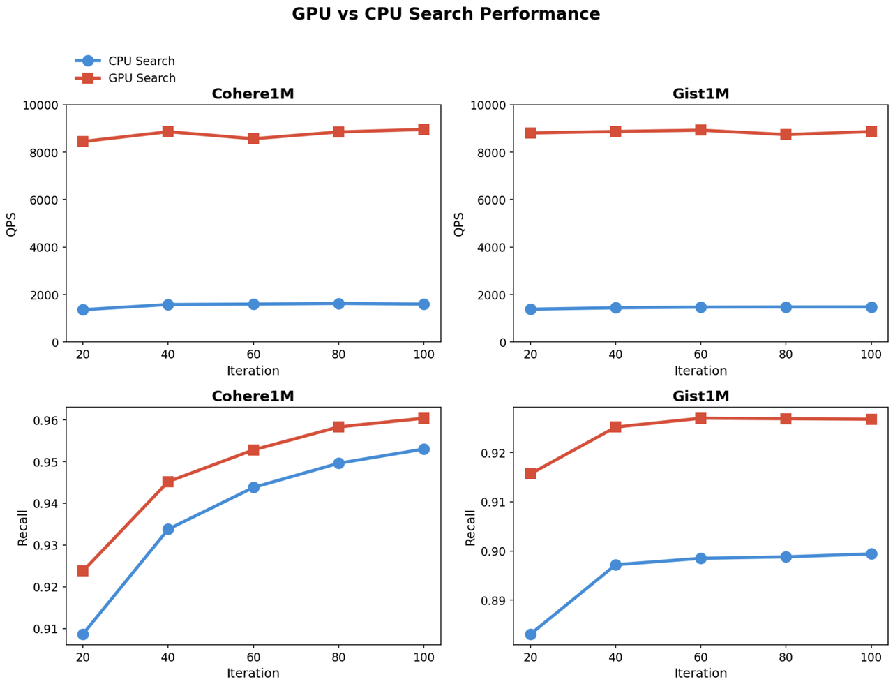
Key Findings

GPU search throughput is 5–6× higher than CPU search. Across both Cohere1M and Gist1M, GPU-based traversal delivers substantially higher QPS, highlighting the efficiency of parallel graph navigation on GPUs.
Recall increases with NN-Descent iterations, then plateaus. As the number of build iterations grows, recall improves for both CPU and GPU querying. However, beyond a certain point, additional iterations yield diminishing gains, indicating that graph quality has largely converged.

3. Recall accuracy

In this experiment, both CAGRA and HNSW are queried on the CPU to compare recall under identical query conditions.

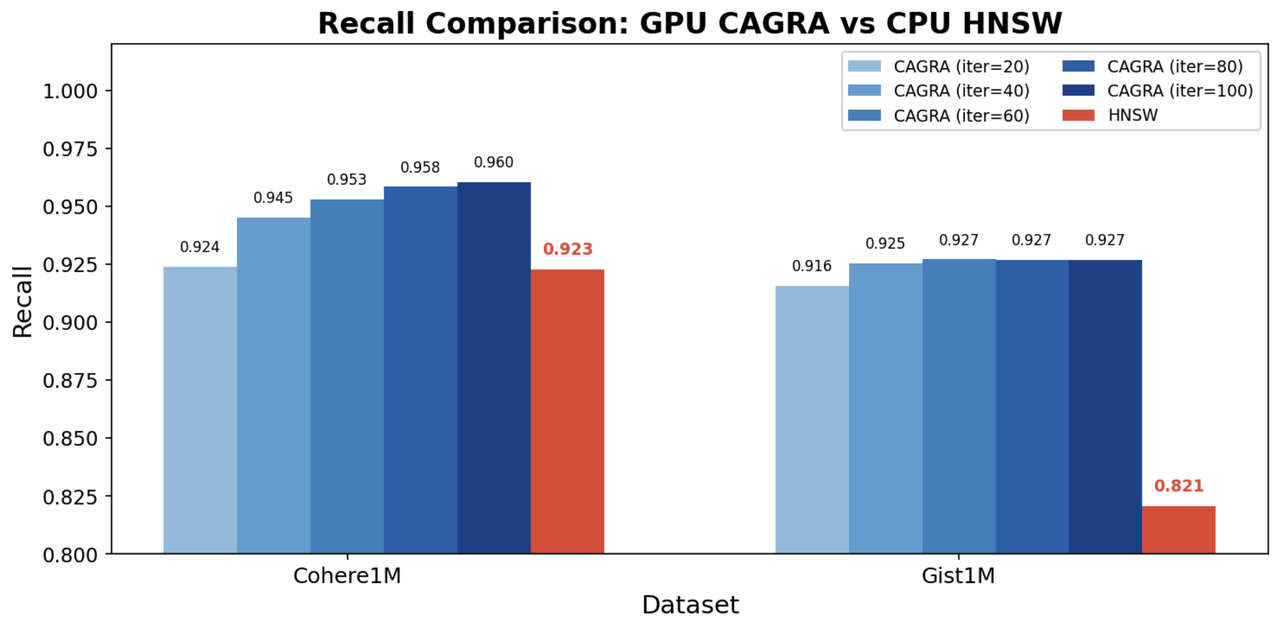
Key Findings

CAGRA achieves higher recall than HNSW on both datasets, showing that even when a CAGRA index is built on the GPU and deserialized for CPU search, the graph quality is well preserved.

What’s Next: Scaling Index Construction with Vamana

Milvus’s hybrid GPU–CPU approach offers a practical and cost-efficient solution for today’s large-scale vector search workloads. By building high-quality CAGRA graphs on GPUs and serving queries on CPUs, it combines fast index construction with scalable, affordable query execution—particularly well suited for workloads with infrequent updates, high query volumes, and strict cost constraints.

At even larger scales—tens or hundreds of billions of vectors—index construction itself becomes the bottleneck. When the full dataset no longer fits into GPU memory, the industry typically turns to insert-based graph construction methods such as Vamana. Instead of building the graph all at once, Vamana processes data in batches, incrementally inserting new vectors while maintaining global connectivity.

Its construction pipeline follows three key stages:

1. Geometric batch growth — beginning with small batches to form a skeleton graph, then increasing batch size to maximize parallelism, and finally using large batches to refine details.

2. Greedy insertion — each new node is inserted by navigating from a central entry point, iteratively refining its neighbor set.

3. Backward edge updates — adding reverse connections to preserve symmetry and ensure efficient graph navigation.

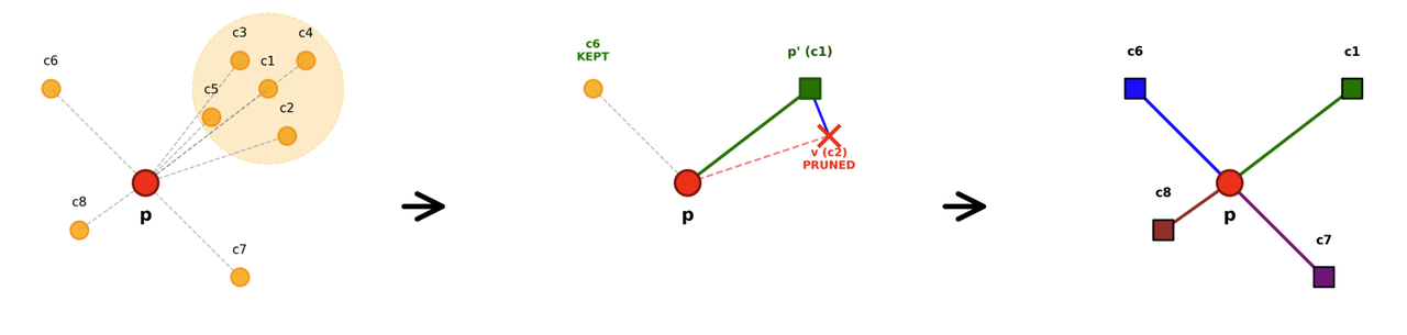
Pruning is integrated directly into the construction process using the α-RNG criterion: if a candidate neighbor v is already covered by an existing neighbor p′ (i.e., d(p′, v) < α × d(p, v)), then v is pruned. The parameter α allows precise control over sparsity and accuracy. GPU acceleration is achieved through in-batch parallelism and geometric batch scaling, striking a balance between index quality and throughput.

Together, these techniques enable teams to handle rapid data growth and large-scale index updates without running into GPU memory limitations.

The Milvus team is actively building Vamana support, with a targeted release in the first half of 2026. Stay tuned.

Have questions or want a deep dive on any feature of the latest Milvus? Join our Discord channel or file issues on GitHub. You can also book a 20-minute one-on-one session to get insights, guidance, and answers to your questions through Milvus Office Hours.