Home
Blog
Introducing AISAQ in Milvus: Billion-Scale Vector Search Just Got 3,200× Cheaper on Memory

Introducing AISAQ in Milvus: Billion-Scale Vector Search Just Got 3,200× Cheaper on Memory

Engineering

December 10, 2025

Martin Li

Vector databases have become core infrastructure for mission-critical AI systems, and their data volumes are growing exponentially—often reaching billions of vectors. At that scale, everything becomes harder: maintaining low latency, preserving accuracy, ensuring reliability, and operating across replicas and regions. But one challenge tends to surface early and dominate architectural decisions—COST.

To deliver fast search, most vector databases keep key indexing structures in DRAM (Dynamic Random Access Memory), the fastest and most expensive tier of memory. This design is effective for performance, but it scales poorly. DRAM usage scales with data size rather than query traffic, and even with compression or partial SSD offloading, large portions of the index must remain in memory. As datasets grow, memory costs quickly become a limiting factor.

Milvus already supports DISKANN, a disk-based ANN approach that reduces memory pressure by moving much of the index onto SSD. However, DISKANN still relies on DRAM for compressed representations used during search. Milvus 2.6 takes this further with AISAQ, a disk-based vector index inspired by DISKANN that stores all search-critical data on disk. In a billion-vector workload, this reduces memory usage from 32 GB to about 10 MB—a 3,200× reduction—while maintaining practical performance.

In the sections that follow, we explain how graph-based vector search works, where memory costs come from, and how AISAQ reshapes the cost curve for billion-scale vector search.

How Conventional Graph-Based Vector Search Works

Vector search is the process of finding data points whose numerical representations are closest to a query in a high-dimensional space. “Closest” simply means the smallest distance according to a distance function, such as cosine distance or L2 distance. At a small scale, this is straightforward: compute the distance between the query and every vector, then return the nearest ones. At a large scale, say billion-scale, however, this approach quickly becomes too slow to be practical.

To avoid exhaustive comparisons, modern approximate nearest neighbor search (ANNS) systems rely on graph-based indices. Instead of comparing a query against every vector, the index organizes vectors into a graph. Each node represents a vector, and edges connect vectors that are numerically close. This structure allows the system to narrow the search space dramatically.

The graph is built in advance, based solely on relationships between vectors. It does not depend on queries. When a query arrives, the system’s task is to navigate the graph efficiently and identify the vectors with the smallest distance to the query—without scanning the entire dataset.

The search begins from a predefined entry point in the graph. This starting point may be far from the query, but the algorithm improves its position step by step by moving toward vectors that appear closer to the query. During this process, the search maintains two internal data structures that work together: a candidate list and a result list.

And the two most important steps during this process are expanding the candidate list and updating the result list.

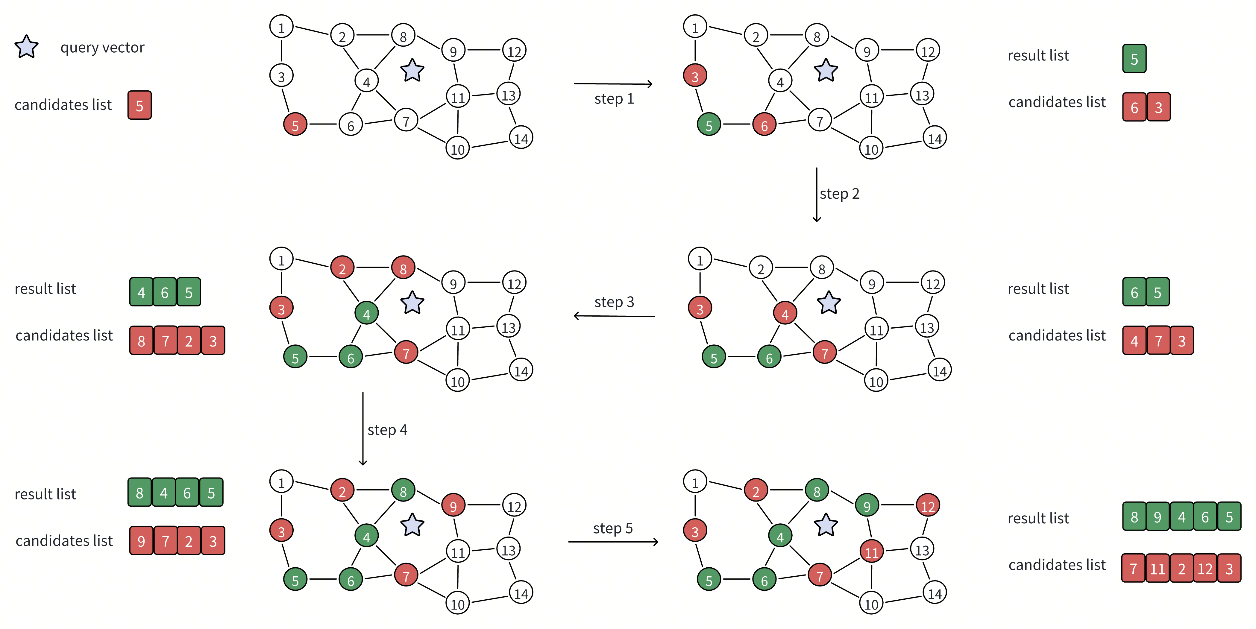
Expanding the Candidate List

The candidate list represents where the search can go next. It is a prioritized set of graph nodes that appear promising based on their distance to the query.

At each iteration, the algorithm:

Selects the closest candidate discovered so far. From the candidate list, it chooses the vector with the smallest distance to the query.
Retrieves that vector’s neighbors from the graph. These neighbors are vectors that were identified during index construction as being close to the current vector.
Evaluates unvisited neighbors and adds them to the candidate list. For each neighbor that has not already been explored, the algorithm computes its distance to the query. Previously visited neighbors are skipped, while new neighbors are inserted into the candidate list if they appear promising.

By repeatedly expanding the candidate list, the search explores increasingly relevant regions of the graph. This allows the algorithm to move steadily toward better answers while examining only a small fraction of all vectors.

Updating the Result List

At the same time, the algorithm maintains a result list, which records the best candidates found so far for the final output. As the search progresses, it:

Tracks the closest vectors encountered during traversal. These include vectors selected for expansion as well as others evaluated along the way.
Stores their distances to the query. This makes it possible to rank candidates and maintain the current top-K nearest neighbors.

Over time, as more candidates are evaluated and fewer improvements are found, the result list stabilizes. Once further graph exploration is unlikely to produce closer vectors, the search terminates and returns the result list as the final answer.

In simple terms, the candidate list controls exploration, while the result list captures the best answers discovered so far.

The Trade-Off in Graph-Based Vector Search

This graph-based approach is what makes large-scale vector search practical in the first place. By navigating the graph instead of scanning every vector, the system can find high-quality results while touching only a small fraction of the dataset.

However, this efficiency does not come for free. Graph-based search exposes a fundamental trade-off between accuracy and cost.

Exploring more neighbors improves accuracy by covering a larger portion of the graph and reducing the chance of missing true nearest neighbors.
At the same time, every additional expansion adds work: more distance calculations, more accesses to the graph structure, and more reads of vector data. As the search explores deeper or wider, these costs accumulate. Depending on how the index is designed, they show up as higher CPU usage, increased memory pressure, or additional disk I/O.

Balancing these opposing forces—high recall versus efficient resource usage—is central to graph-based search design.

Both DISKANN and AISAQ are built around this same tension, but they make different architectural choices about how and where these costs are paid.

How DISKANN Optimizes Disk-Based Vector Search

DISKANN is the most influential disk-based ANN solution to date and serves as the official baseline for the NeurIPS Big ANN competition, a global benchmark for billion-scale vector search. Its significance lies not just in performance, but in what it proved: graph-based ANN search does not have to live entirely in memory to be fast.

By combining SSD-based storage with carefully chosen in-memory structures, DISKANN demonstrated that large-scale vector search could achieve strong accuracy and low latency on commodity hardware—without requiring massive DRAM footprints. It does this by rethinking which parts of the search must be fast and which parts can tolerate slower access.

At a high level, DISKANN keeps the most frequently accessed data in memory, while moving larger, less frequently accessed structures to disk. This balance is achieved through several key design choices.

1. Using PQ Distances to Expand the Candidate List

Expanding the candidate list is the most frequent operation in graph-based search. Each expansion requires estimating the distance between the query vector and the neighbors of a candidate node. Performing these calculations using full, high-dimensional vectors would require frequent random reads from disk—an expensive operation both computationally and in terms of I/O.

DISKANN avoids this cost by compressing vectors into Product Quantization (PQ) codes and keeping them in memory. PQ codes are much smaller than full vectors, but still preserve enough information to estimate distance approximately.

During candidate expansion, DISKANN computes distances using these in-memory PQ codes instead of reading full vectors from SSD. This dramatically reduces disk I/O during graph traversal, allowing the search to quickly and efficiently expand candidates while keeping most SSD traffic out of the critical path.

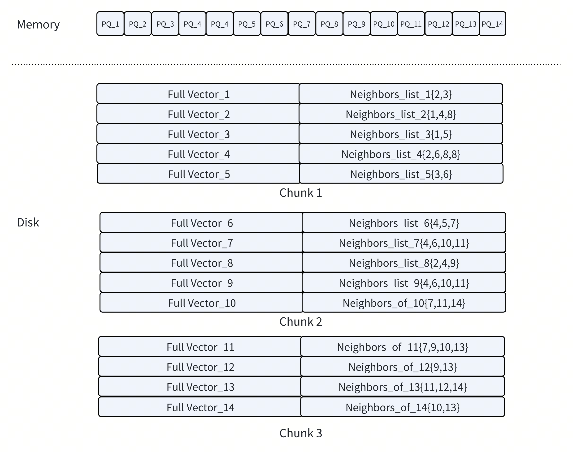
2. Co-Locating Full Vectors and Neighbor Lists on Disk

Not all data can be compressed or accessed approximately. Once promising candidates have been identified, the search still needs access to two types of data for accurate results:

Neighbor lists, to continue graph traversal
Full (uncompressed) vectors, for final reranking

These structures are accessed less frequently than PQ codes, so DISKANN stores them on SSD. To minimize disk overhead, DISKANN places each node’s neighbor list and its full vector in the same physical region on disk. This ensures that a single SSD read can retrieve both.

By co-locating related data, DISKANN reduces the number of random disk accesses required during search. This optimization improves both expansion and reranking efficiency, especially at a large scale.

3. Parallel Node Expansion for Better SSD Utilization

Graph-based ANN search is an iterative process. If each iteration expands only one candidate node, the system issues just a single disk read at a time, leaving most of the SSD’s parallel bandwidth unused. To avoid this inefficiency, DISKANN expands multiple candidates in each iteration and sends parallel read requests to the SSD. This approach makes much better use of available bandwidth and reduces the total number of iterations required.

The beam_width_ratio parameter controls how many candidates are expanded in parallel: Beam width = number of CPU cores × beam_width_ratio. A higher ratio widens the search—potentially improving accuracy—but also increases computation and disk I/O.

To offset this, DISKANN introduces a search_cache_budget_gb_ratio that reserves memory to cache frequently accessed data, reducing repeated SSD reads. Together, these mechanisms help DISKANN balance accuracy, latency, and I/O efficiency.

Why This Matters — and Where the Limits Appear

DISKANN’s design is a major step forward for disk-based vector search. By keeping PQ codes in memory and pushing larger structures to SSD, it significantly reduces the memory footprint compared to fully in-memory graph indexes.

At the same time, this architecture still depends on always-on DRAM for search-critical data. PQ codes, caches, and control structures must remain resident in memory to keep traversal efficient. As datasets grow to billions of vectors and deployments add replicas or regions, that memory requirement can still become a limiting factor.

This is the gap that AISAQ is designed to address.

How AISAQ Works and Why It Matters

AISAQ builds directly on the core ideas behind DISKANN but introduces a critical shift: it eliminates the need to keep PQ data in DRAM. Instead of treating compressed vectors as search-critical, always-in-memory structures, AISAQ moves them to SSD and redesigns how graph data is laid out on disk to preserve efficient traversal.

To make this work, AISAQ reorganizes node storage so that data needed during graph search—full vectors, neighbor lists, and PQ information—is arranged on disk in patterns optimized for access locality. The goal is not just to push more data to the more economical disk, but to do so without breaking the search process described earlier.

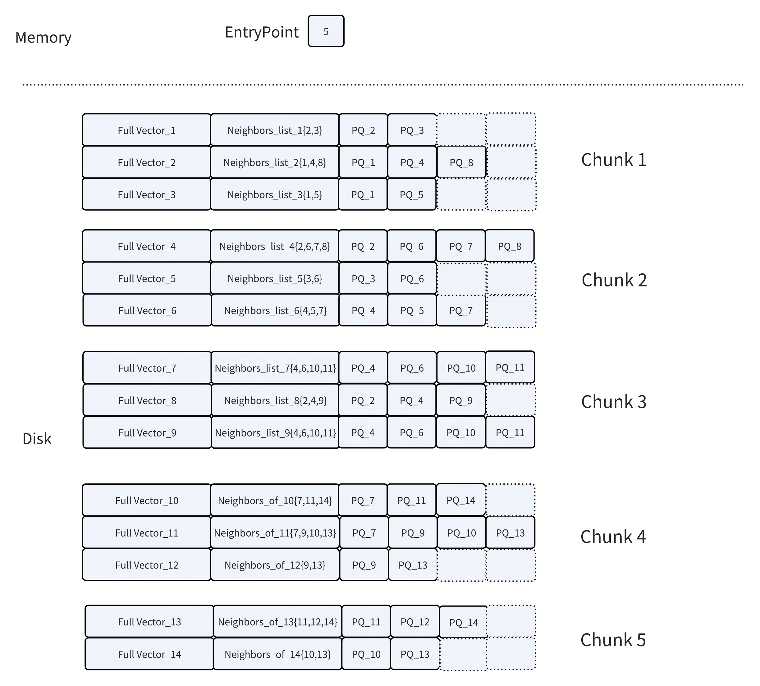
To balance performance and storage efficiency under different workloads, AISAQ provides two disk-based storage modes. These modes differ primarily in how PQ-compressed data is stored and accessed during search.

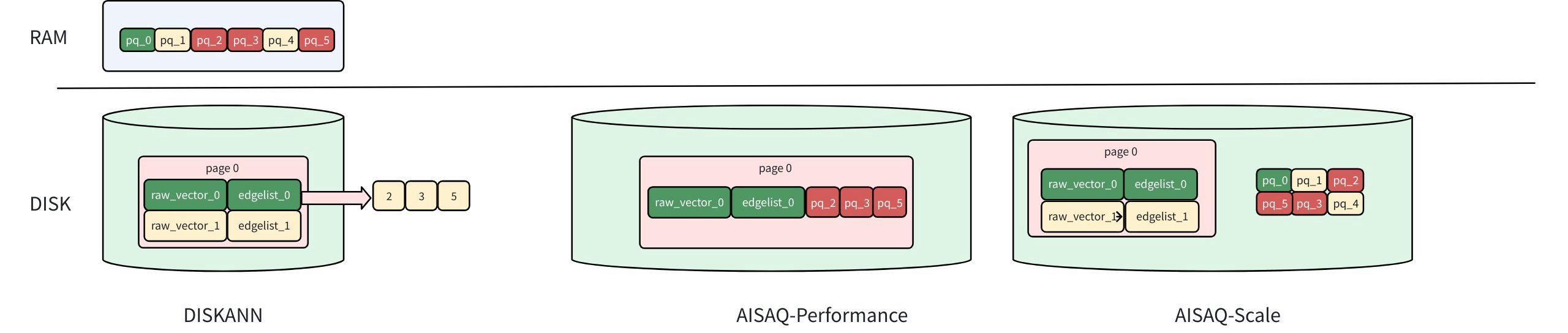
AISAQ-performance: Optimized for Speed

AISAQ-performance keeps all data on disk while maintaining low I/O overhead through data colocation.

In this mode:

Each node’s full vector, edge list, and its neighbors’ PQ codes are stored together on disk.
Visiting a node still requires only a single SSD read, because all data needed for candidate expansion and evaluation is colocated.

From the perspective of the search algorithm, this closely mirrors DISKANN’s access pattern. Candidate expansion remains efficient, and runtime performance is comparable, even though all search-critical data now lives on disk.

The trade-off is storage overhead. Because a neighbor’s PQ data may appear in multiple nodes’ disk pages, this layout introduces redundancy and significantly increases the overall index size.

Therefore, the AISAQ-Performance mode prioritizes low I/O latency over disk efficiency.

AISAQ-scale: Optimized for Storage Efficiency

AISAQ-Scale takes the opposite approach. It is designed to minimize disk usage while still keeping all data on SSD.

In this mode:

PQ data is stored on disk separately, without redundancy.
This eliminates redundancy and dramatically reduces index size.

The trade-off is that accessing a node and its neighbors’ PQ codes may require multiple SSD reads, increasing I/O operations during candidate expansion. Left unoptimized, this would significantly slow down search.

To control this overhead, the AISAQ-Scale mode introduces two additional optimizations:

PQ data rearrangement, which orders PQ vectors by access priority to improve locality and reduce random reads.
A PQ cache in DRAM (pq_cache_size), which stores frequently accessed PQ data and avoids repeated disk reads for hot entries.

With these optimizations, the AISAQ-Scale mode achieves much better storage efficiency than AISAQ-Performance, while maintaining practical search performance. That performance remains lower than DISKANN or AISAQ-Performance, but the memory footprint is dramatically smaller.

Key Advantages of AISAQ

By moving all search-critical data to disk and redesigning how that data is accessed, AISAQ fundamentally changes the cost and scalability profile of graph-based vector search. Its design delivers three significant advantages.

1. Up to 3,200× Lower DRAM Usage

Product Quantization significantly reduces the size of high-dimensional vectors, but at billion scale, the memory footprint is still substantial. Even after compression, PQ codes must be kept in memory during search in conventional designs.

For example, on SIFT1B, a benchmark with one billion 128-dimensional vectors, PQ codes alone require roughly 30–120 GB of DRAM, depending on configuration. Storing the full, uncompressed vectors would require an additional ~480 GB. While PQ reduces memory usage by 4–16×, the remaining footprint is still large enough to dominate infrastructure cost.

AISAQ removes this requirement entirely. By storing PQ codes on SSD instead of DRAM, memory is no longer consumed by persistent index data. DRAM is used only for lightweight, transient structures such as candidate lists and control metadata. In practice, this reduces memory usage from tens of gigabytes to around 10 MB. In a representative billion-scale configuration, DRAM drops from 32 GB to 10 MB, a 3,200× reduction.

Given that SSD storage costs roughly 1/30 the price per unit of capacity compared to DRAM, this shift has a direct and dramatic impact on total system cost.

2. No Additional I/O Overhead

Moving PQ codes from memory to disk would normally increase the number of I/O operations during search. AISAQ avoids this by carefully controlling data layout and access patterns. Rather than scattering related data across the disk, AISAQ co-locates PQ codes, full vectors, and neighbor lists so they can be retrieved together. This ensures that candidate expansion does not introduce additional random reads.

To give users control over the trade-off between index size and I/O efficiency, AISAQ introduces the inline_pq parameter, which determines how much PQ data is stored inline with each node:

Lower inline_pq: smaller index size, but may require extra I/O
Higher inline_pq: larger index size, but preserves single-read access

When configured with inline_pq = max_degree, AISAQ reads a node’s full vector, neighbor list, and all PQ codes in one disk operation, matching DISKANN’s I/O pattern while keeping all data on SSD.

3. Sequential PQ Access Improves Computation Efficiency

In DISKANN, expanding a candidate node requires R random memory accesses to fetch the PQ codes of its R neighbors. AISAQ eliminates this randomness by retrieving all PQ codes in a single I/O and storing them sequentially on disk.

Sequential layout provides two important benefits:

Sequential SSD reads are much faster than scattered random reads.
Contiguous data is more cache-friendly, enabling CPUs to compute PQ distances more efficiently.

This improves both speed and predictability of PQ distance calculations and helps offset the performance cost of storing PQ codes on SSD rather than DRAM.

AISAQ vs. DISKANN: Performance Evaluation

After understanding how AISAQ differs architecturally from DISKANN, the next question is straightforward: how do these design choices affect performance and resource usage in practice? This evaluation compares AISAQ and DISKANN across three dimensions that matter most at a billion scale: search performance, memory consumption, and disk usage.

In particular, we examine how AISAQ behaves as the amount of inlined PQ data (INLINE_PQ) changes. This parameter directly controls the trade-off between index size, disk I/O, and runtime efficiency. We also evaluate both approaches on low- and high-dimensional vector workloads, since dimensionality strongly influences the cost of distance computation and storage requirements.

Setup

All experiments were conducted on a single-node system to isolate index behavior and avoid interference from network or distributed-system effects.

Hardware configuration:

CPU: Intel® Xeon® Platinum 8375C CPU @ 2.90GHz
Memory: Speed: 3200 MT/s, Type: DDR4, Size: 32 GB
Disk: 500 GB NVMe SSD

Index Build Parameters

{
  "max_degree": 48,
  "search_list_size": 100,
  "inline_pq": 0/12/24/48,  // AiSAQ only
  "pq_code_budget_gb_ratio": 0.125,
  "search_cache_budget_gb_ratio": 0.0,
  "build_dram_budget_gb": 32.0
}

Query Parameters

{
  "k": 100,
  "search_list_size": 100,
  "beamwidth": 8
}

Benchmark Method

Both DISKANN and AISAQ were tested using Knowhere, the open-source vector search engine used in Milvus. Two datasets were used in this evaluation:

SIFT128D (1M vectors): a well-known 128-dimensional benchmark commonly used for image descriptor search. (Raw dataset size ≈ 488 MB)
Cohere768D (1M vectors): a 768-dimensional embedding set typical of transformer-based semantic search. (Raw dataset size ≈ 2930 MB)

These datasets reflect two distinct real-world scenarios: compact vision features and large semantic embeddings.

Results

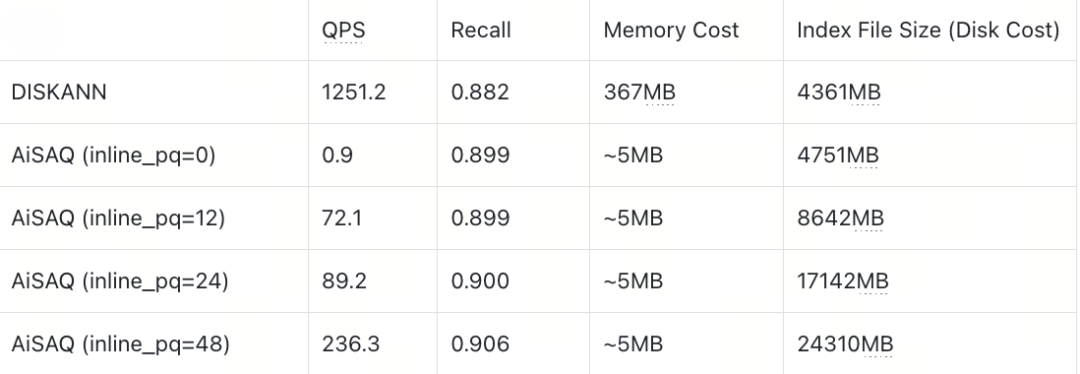
Sift128D1M (Full Vector ~488MB)

Cohere768D1M (Full Vector ~2930MB)

Analysis

SIFT128D Dataset

On the SIFT128D dataset, AISAQ can match DISKANN’s performance when all PQ data is inlined so that each node’s required data fits entirely into a single 4 KB SSD page (INLINE_PQ = 48). Under this configuration, every piece of information needed during search is colocated:

Full vector: 512B
Neighbor list: 48 × 4 + 4 = 196B
PQ codes of neighbors: 48 × (512B × 0.125) ≈ 3072B
Total: 3780B

Because the entire node fits within one page, only one I/O is needed per access, and AISAQ avoids random reads of external PQ data.

However, when only part of the PQ data is inlined, the remaining PQ codes must be fetched from elsewhere on disk. This introduces additional random I/O operations, which sharply increase IOPS demand and lead to significant performance drops.

Cohere768D Dataset

ON the Cohere768D dataset, AISAQ performs worse than DISKANN. The reason is that a 768-dimensional vector simply does not fit into one 4 KB SSD page:

Full vector: 3072B
Neighbor list: 48 × 4 + 4 = 196B
PQ codes of neighbors: 48 × (3072B × 0.125) ≈ 18432B
Total: 21,700 B (≈ 6 pages)

In this case, even if all PQ codes are inlined, each node spans multiple pages. While the number of I/O operations stays consistent, each I/O must transfer far more data, consuming SSD bandwidth much faster. Once bandwidth becomes the limiting factor, AISAQ cannot keep pace with DISKANN—especially on high-dimensional workloads where per-node data footprints grow quickly.

Note:

AISAQ’s storage layout typically increases the on-disk index size by 4× to 6×. This is a deliberate trade-off: full vectors, neighbor lists, and PQ codes are colocated on disk to enable efficient single-page access during search. While this increases SSD usage, disk capacity is significantly cheaper than DRAM and scales more easily at large data volumes.

In practice, users can tune this trade-off by adjusting INLINE_PQ and PQ compression ratios. These parameters make it possible to balance search performance, disk footprint, and overall system cost based on workload requirements, rather than being constrained by fixed memory limits.

Conclusion

The economics of modern hardware are changing. DRAM prices remain high, while SSD performance has advanced rapidly—PCIe 5.0 drives now deliver bandwidth exceeding 14 GB/s. As a result, architectures that shift search-critical data from expensive DRAM to far more affordable SSD storage are becoming increasingly compelling. With SSD capacity costing less than 30 times as much per gigabyte as DRAM, these differences are no longer marginal—they meaningfully influence system design.

AISAQ reflects this shift. By eliminating the need for large, always-on memory allocations, it enables vector search systems to scale based on data size and workload requirements rather than DRAM limits. This approach aligns with a broader trend toward “all-in-storage” architectures, where fast SSDs play a central role not just in persistence, but in active computation and search.

This shift is unlikely to be confined to vector databases. Similar design patterns are already emerging in graph processing, time-series analytics, and even parts of traditional relational systems, as developers rethink long-standing assumptions about where data must reside to achieve acceptable performance. As hardware economics continue to evolve, system architectures will follow.

For more details on the designs discussed here, see the documentation:

Have questions or want a deep dive on any feature of the latest Milvus? Join our Discord channel or file issues on GitHub. You can also book a 20-minute one-on-one session to get insights, guidance, and answers to your questions through Milvus Office Hours.